
At the moment I try to improve my knowledge about functional programming in R. Luckily there are some explanations on the topic in the web (adv-r and Cartesian Faith). Beginning to (re)discover the usefulness of closures, I remember some (at first sight) very strange behaviour. Actually it is consistent within the scoping rules of R, but until I felt to be on the same level of consistency it took a while.
What is a promise?
Every argument you pass to a function is a promise until the moment R evaluates it. Consider a function g with arguments x and y; let’s leave out one argument in the function call:
g <- function(x, y) x
g(1)
## [1] 1R will be forgiving (lazy) until the argument y is actually needed. Until then y exists in the environment of the function call as a ‘name without a value’. Only when R needs to evaluate y a value is searched for. This means that we can pass some non-existent objects as arguments to the function g and R won’t care until the argument is needed in the functions body.
g(1, nonExistentObject)## [1] 1Have a look at the figure ‘Environment Path 1’ (this is the inspiration). Your workspace is also called the Global Environment and you can access it explicitly using the internal variable .GlobalEnv. There is one variable in my workspace, the function g(x, y). When g is called a new environment is created in which it’s body will be evaluated. This is denoted by the solid line. In this new environment of g there exist two variables, x and y. As long as those variables are not needed, no values are bound to those names only a promise that a value can be found at the time of evaluation. Since x is evaluated, the value 1 is bound to x in the environment of the function g. y, however, is not evaluated, so the promised value of y is never searched for and we can promise anything.
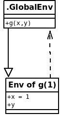
The dashed line indicates the direction in which R will try to find objects. Meaning that if the function g does not find a variable in its own ‘evaluation environment’, it will continue its search in the global environment. The question where this dashed line is pointing to is really important if you try to understand closures. Just to give you a heads up: The parent environment (environment where the dashed line is pointing to) of a ‘functions evaluation environment’ is always the environment in which the function was created – and not the environment from which the function is called. In the case of g that is the global environment. In the case of a function living in a package it is the packages namespace.
What is a closure?
A closure is a function which has an enclosing environment. As far as my understanding of these things goes, by that definition every function can be considered a closure. This suspicion is supported by R’s constant complaint, that I try to subset closures. Anyway, typically the term closure is used for functions which will have a function as return value:
fClosure <- function(p) function(x) x^p
f1 <- fClosure(1)
f2 <- fClosure(2)

cbind(f1(1:10), f2(1:10))
## [,1] [,2]
## [1,] 1 1
## [2,] 2 4
## [3,] 3 9
## [4,] 4 16
## [5,] 5 25
## [6,] 6 36
## [7,] 7 49
## [8,] 8 64
## [9,] 9 81
## [10,] 10 100Here I created fClosure as a function of p which will return a function of x. Then I assign values to f1 and f2 which are the functions \( f(x) = x^1 \) and \( f(x) = x^2 \). The reason this works can be answered by looking at the figure ‘Environment Path 2’ with all environments and connections between them.
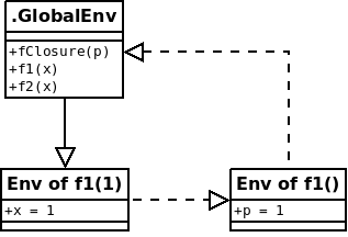
The solid line indicates that f1 is called from the .GlobalEnv; the dashed line the direction in which R will search for values (an exception is the promise, x, which will reference to the .GlobalEnv). The enclosing environment of f1 is the environment in which it was created, which was the environment of the call to fClosure. So f1 has an own environment which can be seen when you print the function to the console.
f1## function(x) x^p
## <environment: 0x24488e8>This environment can even be accessed, to check what is going on inside.
ls(environment(f1))## [1] "p"get("p", envir = environment(f1))## [1] 1So in the enclosing environment of f1 lives a variable p with value 1. Whenever R searches for a variable which is not part of the argument list, it will first check the environment created when called, then the enclosing environment and then the .GlobalEnv followed by the search path.
Why are those two related?
When I read about the scoping rules in R I never really understood the implications of the word lazy. It needed a couple of hours of utter confusion and experiments with closures that I got it. Consider the case where I want to construct an arbitrary number of functions like in the above example. Copy-pasting fClosure will quickly reach limits and is more frustrating than coding.
# Creating f1-f5 and store them in a list
# This will actually work using lapply in the most recent R version (3.2)
# I enforce it by using a for-loop instead of lapply...
# funList <- lapply(1:5, fClosure)
funList <- list()
for (i in 1:5) funList[[i]] <- fClosure(i)
# Call f1-f5 with the argument x = 1:10
resultList <- lapply(funList, do.call, args = list(x = 1:10))
# Cbind the results
do.call(cbind, resultList)
## [,1] [,2] [,3] [,4] [,5]
## [1,] 1 1 1 1 1
## [2,] 32 32 32 32 32
## [3,] 243 243 243 243 243
## [4,] 1024 1024 1024 1024 1024
## [5,] 3125 3125 3125 3125 3125
## [6,] 7776 7776 7776 7776 7776
## [7,] 16807 16807 16807 16807 16807
## [8,] 32768 32768 32768 32768 32768
## [9,] 59049 59049 59049 59049 59049
## [10,] 100000 100000 100000 100000 100000Ups, what happened? The resulting matrix looks like every column was created using the same function! Just to be clear, the above code works just fine. It does exactly as intended. In this case I was tricked by the promises in the enclosing environments, and that in those enclosing environments there live variables p with values 1 to 5. This is not so. Remember, the arguments of a function are evaluated when they are first needed. Until then they are promises. The concept of a promise was surprising because it’s one of the very few objects which have reference semantics in base-R. So a promise is just a pointer to a variable name in an environment (the environment from which the function is called) – they are not pointing to values! If the value of the variable pointed to changes before the promise is evaluated inside the function, the behaviour of the function will change too. This leads to the question: what is the value of p inside this list of functions?
sapply(funList, function(fun) get("p", envir = environment(fun)))## [1] 5 5 5 5 5Okay, fine, so in the loop where I created the functions f1 to f5, I did pass the numbers 1 to 5 to the closure, however, they do not get evaluated but point to the iterator which is 5 at the moment the promises are evaluated. How do we fix this? Evaluate p in the enclosing environment at the moment of assignment. Actually we could just write p in the functions body (not the function which is returned, it needs to be evaluated in the enclosing environment), but that may be considered bad style because in two weeks time you will see it as a redundant and useless line of code. Actually there is a function for this. force forces the evaluation of arguments in the enclosing environment. This means that the variable p will be bound to a value at the moment the closure is called.
# Fix
fClosure <- function(p) {
  force(p)
  function(x) x^p
}

# And again, with a new definition of fClosure:
for(i in 1:5) funList[[i]] <- fClosure(i)
resultList <- lapply(funList, do.call, args = list(x = 1:10))
do.call(cbind, resultList)
## [,1] [,2] [,3] [,4] [,5]
## [1,] 1 1 1 1 1
## [2,] 2 4 8 16 32
## [3,] 3 9 27 81 243
## [4,] 4 16 64 256 1024
## [5,] 5 25 125 625 3125
## [6,] 6 36 216 1296 7776
## [7,] 7 49 343 2401 16807
## [8,] 8 64 512 4096 32768
## [9,] 9 81 729 6561 59049
## [10,] 10 100 1000 10000 100000And that made all the difference.